Beyond semantic search: Architecting the multi-vector RAG stack in 2026

In the early days of the generative AI boom, semantic search was hailed as the definitive solution for knowledge retrieval. By 2026, however, the industry has reached a “vector plateau”. Simple text-matching is no longer a competitive advantage; it is a legacy baseline. Today’s high-stakes applications—from financial forensics to real-time regulatory monitoring—require a sophisticated orchestration of multiple vector types that encode not just what a piece of data “means,” but how it behaves, who it connects to, and how it evolves over time.

To build resilient AI systems, architects must move beyond the naive Retrieval-Augmented Generation (RAG) models of the past. Understanding the nuances of the modern vector landscape is the first step toward solving “AI amnesia” and achieving industrial-grade precision. Before diving into the complexities of hybrid architectures, it is essential to understand the foundational role of the Vector Database in AI and RAG Models.

---

The 2026 vector taxonomy: From meanings to behaviors

The traditional approach to vectorization relied almost exclusively on dense NLP embeddings—continuous numerical arrays that approximate conceptual similarity. While these are excellent for finding synonyms, they are notoriously poor at handling exact keywords, structural relationships, or temporal sequences.

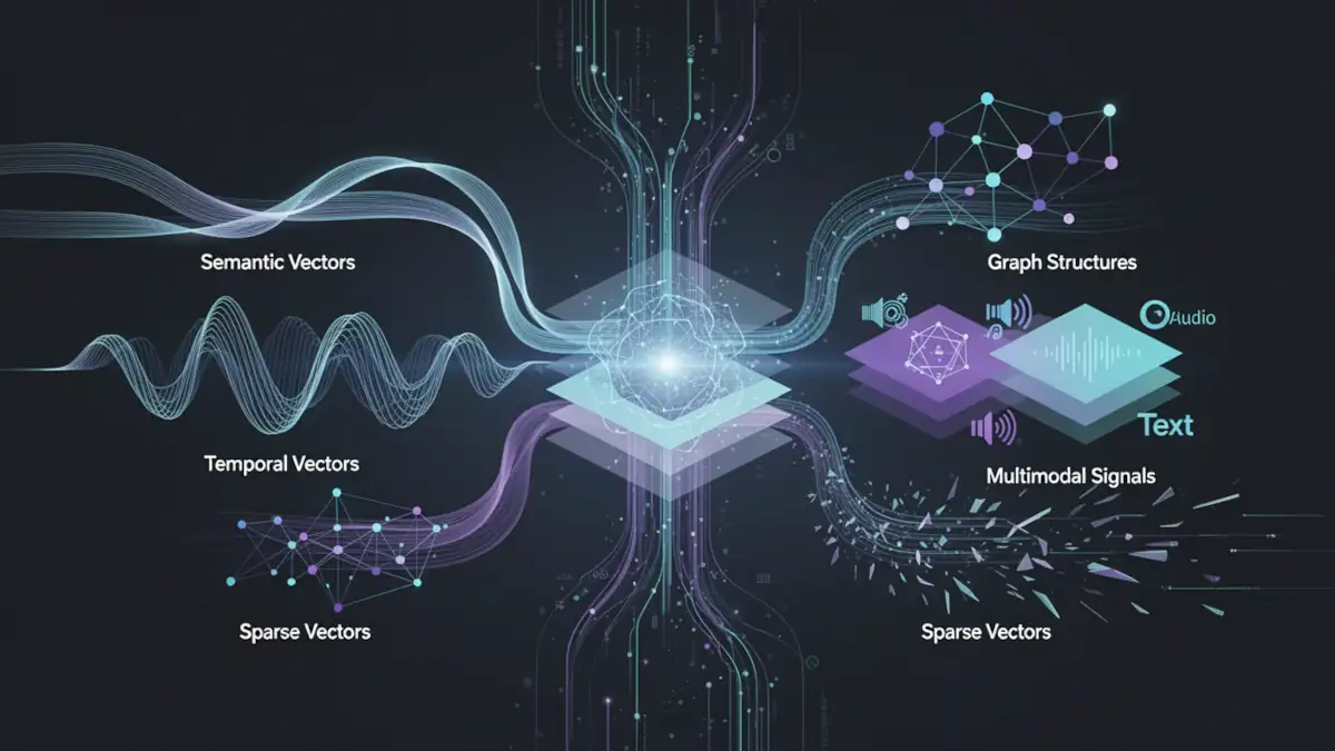
The “Precision Paradox” of 2026 is that the more semantically capable our models become, the more they struggle with the specific, rigid facts of the physical world. A purely semantic vector can conflate documents that share topical vocabulary but carry opposite real-world implications—for example, a query about a rare adverse drug event may surface anti-vaccine content because both co-occur with the same clinical terminology. The embedding model captures co-textual proximity, not causal or normative direction. To bridge this gap, modern retrieval architectures now utilize five distinct classes of vectors.

1. Semantic and sparse (The hybrid bedrock)

By combining dense embeddings with learned sparse models like SPLADE or BGE-M3, systems can simultaneously capture conceptual nuance and lexical exactness. BM25-style sparse retrieval guarantees exact-match recall for specific technical terms and product IDs; SPLADE adds controlled term expansion to cover synonyms without sacrificing keyword anchoring. Together, they suppress “semantic drift” in retrieval without relying on any single representation.

2. Temporal vectors (The pulse)

Using Time2Vec or TS2Vec, engineers encode the periodicity and “shape” of events rather than just treating time as a linear metadata filter. This allows an AI to recognize a “DDoS-shaped” traffic spike or a “fraud-shaped” transaction sequence by analyzing the geometric similarity of the time-series itself.

3. Multimodal vectors (The senses)

Unified models like Gemini Embedding 2 or WAVE project text, images, audio, and video into a single shared mathematical space. This enables “direct document RAG,” where the AI can query the visual layout of a PDF page as an image embedding, bypassing the errors inherent in traditional OCR pipelines.

4. Graph embeddings (The network)

Structural models like GraphSAGE encode a node’s position and its neighbors into a vector. This is the “guilt by association” vector, crucial for identifying money-laundering rings where individual actors appear legitimate but their connectivity patterns are toxic.

5. Binary and quantized vectors (The scale)

As datasets reach the petabyte scale, high-precision float vectors become a memory liability. Product Quantization (PQ) and binary codes compress these vectors to a fraction of their size, enabling billion-scale search on edge hardware with minimal recall loss.

Table 1: Vector taxonomy matrix (2026)

Vector type	Core technology	Primary use case	Key limitation
Semantic	BERT, OpenAI v4, Jina	General RAG & Search	Domain/Temporal Drift
Temporal	Time2Vec, TS2Vec	Anomalies & Forecasting	Windowing Granularity
Multimodal	Gemini Embedding 2, WAVE	Video Search & Content Safety	High Compute Cost
Graph	GraphSAGE, R-GCN	Fraud & Social Networks	Structural Opacity
Sparse	SPLADE, BM25	Exact Keywords & Acronyms	Lacks Semantic Context

---

Engineering the modern RAG pipeline: The three-stage retrieval

In 2026, the architectural standard for high-precision retrieval has moved beyond a single “top-k” lookup. Production-grade systems now employ a multi-stage pipeline designed to balance the broad recall of semantic search with the surgical precision required for enterprise data. This pipeline typically consists of three distinct phases: Hybrid Retrieval, Score Fusion, and Reranking.

Stage 1: Hybrid retrieval (Dense + Sparse)

To mitigate the inherent weaknesses of purely semantic models, modern architectures perform parallel searches using both dense and sparse vectors.

• Dense Retrieval: Uses Bi-Encoders to find conceptually related documents within a continuous vector space.
• Sparse Retrieval: Utilizes lexical models like BM25 or learned sparse encoders (SPLADE) to ensure that specific product IDs, acronyms, or technical terms are not lost in the “semantic soup.”

Many leading providers have streamlined this through cascading retrieval, which unifies these signals into a single ingestion and query workflow.

Stage 2: Hybrid scoring and fusion

Once the initial candidates are retrieved, their scores—often calculated using different metrics like Cosine Similarity for dense and Dot Product for sparse—must be unified. The most robust method used today is Reciprocal Rank Fusion (RRF). RRF prioritizes documents that appear consistently at the top of both retrieval lists, effectively filtering out “semantic hallucinations” that only exist in the dense space.

Stage 3: The reranking revolution

The final, and perhaps most critical, stage is Reranking. While the initial retrieval (Bi-encoders) is fast and efficient, it lacks a deep understanding of the query-document interaction.

• The Mechanism: A Cross-Encoder or a specialized Reranker LLM processes a smaller subset of results (the top 50–100) to perform a granular, token-to-token comparison.
• The Performance Gain: Independent benchmarks and production case studies consistently report a 20–40% improvement in retrieval quality after adding a cross-encoder reranking stage. A 2026 study on bi-encoder top-100 followed by cross-encoder reranking to top-10 measured +33–40% RAG answer accuracy gains at a GPU latency cost of approximately 120 ms when batched. Practitioner deployments report similar 20–35% lifts in answer quality at a latency budget of 200–500 ms per query.
• The Trade-off: The cost of this precision is latency. Cross-encoders are significantly more computationally expensive than Bi-encoders, making them unsuitable for the initial search across millions of documents but perfect for the final refinement. LLM-based rerankers push accuracy further but add 800–1,500 ms and significant token costs, making them appropriate for offline evaluation or high-value escalation paths rather than every query.

Table 2: Modern RAG pipeline stages

Stage	Technology	Focus	Latency budget
Retrieval	Bi-Encoders + BM25	Recall (Top 1000)	Milliseconds
Fusion	RRF / Hybrid Scoring	Calibration	Microseconds
Reranking	Cross-Encoders / LLM	Precision (Top 10)	Tens to Hundreds of ms
Generation	Frontier LLMs	Synthesis	Seconds

---

Chunking strategy: The underrated system lever

Before documents reach the retrieval pipeline, they must be segmented into chunks. This seemingly low-level decision is in fact one of the most consequential architecture choices in a RAG system—and one of the most frequently underestimated.

Fixed-size chunking: Why defaults fail

A 2025 systematic study on chunk size across multiple QA datasets revealed a stark split in behavior:

• For short, fact-based QA (SQuAD-style), small chunks of 64–128 tokens maximize Recall@1. Larger chunks dilute the signal and drop recall by 10–15%.
• For long, dispersed-answer datasets (NarrativeQA, TechQA), recall improves dramatically with large chunks of 512–1,024 tokens. On TechQA specifically, Recall@1 rises from 4.8–16.5% at 64–128 tokens up to 61–71% at 512–1,024 tokens.

The practical implication: blindly applying the “256-token default” is not a neutral choice. It is a systematic regression for any corpus with long-form, multi-section reasoning.

Late chunking: Preserving cross-chunk context

Long-context embedding models have enabled a new approach called late chunking, described in the Weaviate engineering blog and in the original Jina AI research paper. The mechanism works as follows:

1. The full document is encoded by a long-context transformer, allowing each token’s representation to attend to the entire document.
2. The resulting token embeddings are sliced into chunks after the encoder, but before pooling.
3. Each chunk vector therefore carries cross-document context rather than being encoded in isolation.

This approach preserves narrative coherence and section relationships that naive independent chunk embeddings lose. Initial benchmarks show consistent gains as document length grows—particularly for technical documentation, legal contracts, and multi-section reports. Weaviate’s multi2multivec module and Jina’s jina-embeddings-v3 both support late chunking natively.

Practical recommendations

• Tune chunk size per corpus and task, not globally. A 256-token default is appropriate for short-answer search but damaging for long-document retrieval.
• Apply 10–15% token overlap between chunks to avoid context gaps at boundaries; respect logical section breaks (headings, paragraphs) rather than hard token counts.
• Consider parent-child retrieval as a complement to late chunking: index small child chunks for precision, but retrieve the parent passage (800–1,500 tokens) to feed the generator with richer context.

---

Strategic decision: RAG vs. long-context LLMs

In 2026, the rise of models with context windows exceeding one million tokens has sparked a fundamental debate: is RAG still necessary? While long-context (LC) models allow for the ingestion of entire libraries in a single prompt, they do not replace RAG; rather, they redefine the architectural boundaries of where retrieval ends and reasoning begins.

Performance vs. unit cost: The architectural arbitrage

The primary differentiator between RAG and LC is the economic and operational profile of the system. RAG functions as a high-efficiency external memory, while LC serves as a high-density internal reasoning space.

• RAG Cost Profile: High upfront cost for ingestion, embedding, and indexing, but significantly lower marginal costs per query. Benchmark comparisons show RAG pipelines averaging approximately 1 second of end-to-end latency at a cost of around $0.00008 per query.
• Long-Context Cost Profile: Near-zero ingestion cost, but explosive query costs that scale with sequence length. At 200k+ tokens, per-query costs can reach $0.10 or more—a roughly 1,000× difference. At one million tokens, first-token latency can exceed 20–45 seconds depending on infrastructure.

Architects must decide between the “pay-now” model of RAG and the “pay-as-you-go” model of LC. For massive, dynamic datasets, RAG remains the only viable path to maintain predictive analytics and business intelligence without bankrupting the inference budget.

Handling AI amnesia: Why scale still requires RAG

Despite massive context windows, LC models suffer from the “lost in the middle” phenomenon, where the model’s attention accuracy degrades as context size increases. RAG mitigates this “AI amnesia” by delivering only the most relevant “needles” to the LLM’s reasoning “haystack.” This is particularly critical when dealing with Context Packing vs. RAG, where hardware constraints often limit the practical utility of massive contexts in production environments.

The emerging hybrid: RAG + long context + KV caching

The binary framing of “RAG vs. LC” is itself becoming outdated. Many 2025–2026 production stacks adopt a combined approach:

• RAG handles the majority of traffic: routine queries retrieve 1,500–5,000 tokens and pass them to a standard context window.
• Long-context + KV caching handles rare deep-dive analysis: for infrequent, high-value tasks, systems reuse cached KV tensors across requests with shared prefixes, cutting time-to-first-token by 2–3× and increasing throughput significantly—without paying the full recomputation cost on every call.

The practical rule of thumb emerging from independent analyses: for corpora beyond approximately one million tokens queried frequently, RAG is almost always more economical. For small, low-frequency corpora where engineering simplicity matters more, long-context without retrieval remains viable.

Table 3: RAG vs. Long-Context (LC) Trade-offs

Feature	RAG	Long-Context (LC)
Data Scale	Billions of documents	Millions of tokens
Ingestion Cost	High (Indexing/Storage)	Zero (Direct input)
Query Latency	~1 s p95 (fast retrieval)	20–45 s at 1M tokens
Query Cost	~$0.00008 per query	~$0.10+ per query at 200k tokens
Update Frequency	Near-real-time (Index update)	Instant
Reasoning Depth	Fragmented	Holistic/Deep

Concrete Example: Imagine a legal firm auditing 10,000 historical contracts (roughly 50 million tokens).

• Using Long-Context alone would require multiple separate prompts at a massive cost per query, and the model would struggle to maintain cross-document consistency.
• Using RAG, the system indexes the corpus once. Queries can then pinpoint specific clauses across all 10,000 documents in milliseconds for a fraction of the cost, as detailed in the Meilisearch guide on RAG vs Long-Context LLMs.

---

Infrastructure trade-offs: Memory, latency, and indexing

Building a vector-based architecture in 2026 is no longer just about choosing an embedding model; it is about engineering the storage and retrieval layer to survive the “curse of dimensionality” at scale. As datasets migrate from millions to billions of vectors, the choice of indexing algorithm becomes the primary driver of operational cost and system responsiveness.

Choosing your scaling path: HNSW, IVF, and DiskANN

The industry has converged on three primary indexing strategies, each representing a specific compromise between speed, memory usage, and storage media:

• HNSW (Hierarchical Navigable Small World): The gold standard for low-latency retrieval. By building a multi-layered graph of vectors, HNSW allows for incredibly fast traversal across the vector space. However, the entire graph must reside in RAM—benchmarks show memory overheads of 1.5–2.5× the raw vector size for typical configurations—making it prohibitively expensive for billion-scale datasets. At high concurrency, HNSW can also hit out-of-memory ceilings before IVF or DiskANN alternatives.
• IVF (Inverted File Index): A clustering-based approach that partitions the vector space into Voronoi cells. During a search, only the most relevant clusters are probed. IVF is significantly more memory-efficient than HNSW and is often paired with PQ to further reduce its footprint. The trade-off is more complex tuning (nlist, nprobe, codebook size) and a lower maximum recall ceiling.
• DiskANN: The modern solution for massive scale. DiskANN stores the bulk of the index on high-speed NVMe SSDs rather than RAM. Independent benchmarks show DiskANN achieving up to 3.2× higher throughput and 44.5% lower latency than IVF in some configurations at large scale, while remaining 7.7–50.8% slower than HNSW at P99 on moderate-scale workloads. For datasets in the billions of vectors, this trade-off typically favors DiskANN strongly on cost-per-query.

Compression engineering: Quantization as a necessity

To handle the high-dimensional vectors typical of 2026 (often 1,536 to 4,096 dimensions), compression is no longer optional. Techniques like Scalar Quantization (SQ) and Product Quantization (PQ) allow architects to shrink vector sizes significantly:

• Scalar Quantization (INT8/FP16): Reduces the precision of each dimension (e.g., from Float32 to INT8), typically cutting memory usage by 4× with minimal accuracy loss—particularly when paired with cross-encoder reranking that compensates for any quantization-induced recall degradation.
• Product Quantization (PQ): A more aggressive technique that splits vectors into sub-vectors and quantizes them against a learned codebook. PQ can reduce memory requirements by 4–16× or more, but introduces a “quantization error” that must be mitigated through careful parameter tuning and periodic codebook retraining as the data distribution evolves.

Moving from Float32 to Float16 alone halves storage with negligible recall impact for most RAG workloads—making it a low-risk, high-return default for any production deployment.

Table 4: Vector Indexing Trade-offs (2026)

Index Type	Primary Media	P99 Latency	Scalability	RAM Intensity
HNSW	RAM	Ultra-Low	Millions	Very High (1.5–2.5× raw size)
IVF-PQ	RAM / Disk	Medium	Hundreds of millions	Moderate
DiskANN	NVMe SSD	Moderate	Billions	Low
Flat	RAM / Disk	Very High	Archive only	Low

---

Production patterns: Selecting the right vector engine

In 2026, the “best” vector database is determined by your specific architectural pattern rather than raw feature counts. The market has matured into specialized niches that cater to different engineering philosophies.

Architecture patterns for the 2026 stack

Pinecone: The Serverless Cascading Leader Pinecone has optimized for the “developer-first” experience, focusing on cascading retrieval. By unifying dense and sparse signals into a single managed pipeline, it removes the operational burden of manual score fusion.

Qdrant: The Edge and Filtering Specialist Built in Rust, Qdrant excels in environments where strict metadata filtering (e.g., geo-fencing or complex boolean logic) is as important as vector similarity. Its efficiency makes it the preferred choice for edge deployments and high-throughput filtering.

Milvus: The Industrial Scale Powerhouse Designed as a cloud-native distributed system, Milvus is built for the “Billion-Vector” club. It offers the most granular control over index types (HNSW, IVF, DiskANN) and is the most robust option for teams managing their own high-capacity infrastructure.

Weaviate: The Multimodal Modularist Weaviate prioritizes the “Object-Vector” relationship, treating vectors as properties of a data object. Its pluggable module system—enabling native vectorization and late chunking—makes it the most flexible choice for multimodal RAG and complex document processing.

---

Governance and explainability: The case for sparse-dense auditing

One of the most persistent technical hurdles in 2026 remains the “Explainability Gap” inherent in high-dimensional vector spaces. While dense, multimodal, and graph embeddings offer unparalleled depth, they function as mathematical “black boxes,” making it nearly impossible to explain why two items were deemed similar. This lack of transparency poses a significant risk for regulated industries—such as finance and public safety—where every automated decision must be auditable.

The interpretability paradox

The industry has turned to hybrid architectures to solve this governance crisis. Unlike their dense counterparts, sparse lexical vectors (such as BM25 or SPLADE) are inherently interpretable because they map directly to specific terms or tokens. By layering sparse vectors over dense ones, architects can provide a human-readable “justification” for search results.

• Dense Vectors: Capture the “intuition” or conceptual context of the data.
• Graph/Temporal Vectors: Capture the “behavior” and “relational” patterns.
• Sparse Vectors: Provide the “evidence” or specific keyword triggers for the decision.

Case study: Banking audit and money laundering

Consider a financial institution using Graph Neural Networks (GNNs) to identify money-laundering rings. The system generates a graph embedding that flags a specific account because its structural position within a hub-and-spoke network matches known illicit patterns.

When a regulator demands an explanation, a purely dense or graph-based system would struggle to provide one. However, by utilizing a hybrid stack, the system can point to the sparse lexical layer to identify exactly which entity names or specific transaction IDs triggered the initial suspicion, while the temporal vector highlights the anomalous “cadence” of the transfers. This multi-layered approach transforms a “black box” alert into an actionable forensic report, a concept central to modern conversational AI and predictive analytics.

---

Conclusion: Toward adaptive retrieval architectures

As we navigate the complexities of 2026, the strategic imperative has shifted from selecting a “database” to architecting a comprehensive Vector Strategy. The era of the single-vector RAG model is over, replaced by a sophisticated orchestration of semantic, temporal, and structural data types that can scale to billions of entries while maintaining surgical precision.

The next frontier lies in adaptive retrieval pipelines—systems that dynamically select the optimal retrieval strategy based on query characteristics. Rather than treating every query identically, these architectures route requests through different paths:

• Keyword-heavy queries (product IDs, entity names, regulations) are fast-pathed through sparse-first retrieval with minimal reranking overhead.
• Conceptual or exploratory queries leverage dense hybrid retrieval with full cross-encoder reranking.
• Structured or temporal queries invoke graph or time-series vector indexes before merging results with semantic candidates.
• High-stakes or ambiguous queries escalate to LLM-based reranking or trigger a long-context pass with KV cache reuse for deeper reasoning.

This adaptive layer is not yet a standard product feature—it is assembled from orchestration frameworks, routing logic, and evaluation harnesses. But it represents the direction that high-performance RAG systems are moving toward: pipelines that observe, measure, and self-adjust rather than pipelines that simply execute a fixed sequence.

By integrating these diverse mathematical representations within an adaptive routing layer, organizations can finally solve the problem of “AI amnesia” and build systems that truly understand the multidimensional reality of their data. The goal in 2026 is no longer just retrieval; it is retrieval that knows what kind of retrieval the question deserves.

---